Kele Blog - Page 25 of 31

Kele’s UL Panel Shop: Your Source for Meeting Code

Posted on February 8, 2016February 9, 2022 by Kele Inc

Did you know that when you assemble power supplies, controllers, relays, transmitters, and all that other stuff into an enclosure for your control panel, there’s a rule in the NEC that requires your panel to be listed and labeled as an industrial control panel?

Article 409 of the NEC is devoted to the installation of industrial control panels, which are defined as an assembly of two or more components consisting of:

Power circuit components only, such as motor controllers, overload relays, fused disconnect switches, and circuit breakers;
Control circuit components only, such as pushbuttons, pilot lights, selector switches, timers, switches, control relays; or,
A combination of power and control circuit components.

Articles 100 and 110 of the NEC further insist on listed and labeled equipment where such safety standard exists. An informational note in Article 409 refers the installer to UL 508A as an example of a suitable safety standard for industrial control panels. Kele’s UL 508A panel shop can fulfill your needs for a listed and labeled industrial control panel. Send us those drawings in whatever format you choose, and we can help make your panel conform.

So what is UL 508A all about? It’s all about safety – safety from fire, and safety from personal injury. The standard stipulates everything from enclosure type to wire size. There’s a lengthy part about proper separation of power circuits from Class 2 circuits. There are standards that must be met for every part installed in the panel that is upstream of Class 2 circuits. There are labeling requirements for many different scenarios. There are requirements for overcurrent protection and short circuit protection. In sum, a UL 508A panel is a safe panel.

Why Kele? Our UL Panel shop is authorized by UL to list and label your panel as meeting UL 508A standards. Our staff is regularly trained, and a UL inspector makes sure that our work is up to snuff.

We have recently added an additional 1,800 square feet to our panel shop, for a total of 6,720 square feet.

This means we have the capacity to handle your largest projects.

See below for some pictures. We currently have 23 people on our Panel Team with over 150 years on combined experience in BAS/panel building. We’ve also added a new Panel Review Team that will inspect all panel drawings before the panels are moved into production to eliminate any issues or questions plus a Panel Shop Manager, Lisa Bennett, who will make sure your panel is built to spec, on-time and tested before it ships to you, ready to install.

Call Bennie Crowder today at 888-397-5353 or email us at panels@kele.com to get your control panel UL listed. We’ll build it up to the standard, test it, and ship it to you ready to install. Our normal lead time for building panels is 2 weeks or less plus there is an expediting option for quicker shipment. For more information on our panel shop, please visit http://www.kele.com/panel-shop/.

Kele Customers Have Spoken and the Water Detector Family Has Grown

Posted on January 15, 2016 by Kele Inc

Selling a service is selling the intangible. You know, as a consumer, if you are getting great service from a business. You can feel it, but sometimes it’s hard to actually define. Many times, listening to a demand, a complaint, or a request is all that’s needed to provide great service. In product management circles, Voice of the Customer (VoC) is one of the most important drivers in product development. If we LISTEN really well, the solution has already been provided for us. If a customer says, “I wish you had a widget that would do this.” Or “I need a product to do this for me”. When you hear those statements, LISTEN, and take good notes.

Ascertaining VoC can be a challenge for many companies. How can you systemically listen to thousands of “I wish” or “I need” statements and boil it down to a working product development list? At Kele we actually utilize a very modern marketing department to help cultivate customer responses and needs. Using digital media and short surveys gives the product management team at Kele a gateway to thousands of customer voices and opinions. We sort through them quickly and this VoC gives us solutions to provide better products and better services to you the consumer. Of course it takes your participation in the surveys and you, our customer base, have been great about providing your preferences.

One example, is the Kele Water Detector (WD) family expansion project that is launching at the 2016 AHR Expo in Orlando. Kele has provided a legacy water detector device for over 20 years, and continues to serve a wide range of customers. We started to get “I Wish” responses from WD users like this:

I really like your WD product but I WISH you had a poly material (plastic) enclosure option.

I WISH it had a cable option that could bend around corners in the long sensor run.

We literally sorted through hundreds of survey responses. This form of VoC (your responses) helped shape the design requirements for the next generation of Kele water detectors. Our offering has expanded significantly. We also understood through VoC that our legacy WD product is a great product, and is still required by the industry. So many times, product launches involve a planned obsolescence of existing part numbers. In this case customers spoke, no obsolescence is planned, only expansion of a strong product legacy. So thank you for the feedback, we will continue to provide great customer service, and LISTEN.

Are You a Victim of Contractor Compounding?

Posted on December 14, 2015 by Kele Inc

In the financial world, compounding is a good thing, but in the contracting world, it can be your enemy. See if this sad tale we constantly hear from our customers sounds familiar.

Work is up, and you have a lot of parts to order. After tons of phone calls and Web searches, you locate the parts you need and place purchase orders with all the different sources. So far, so good. But then the parts start to rain in from everywhere. You’re getting multiple shipments because you bought from multiple sources. Most vendors today stock little or nothing, so each one sends what they can when they can. Meanwhile, you have to receive those parts, check them in, and decide what to do with them—taking time and effort you don’t have to spare, especially if you’re trying to do it on the job site.

And it just gets worse. You start to get partial invoices from all those compound shipments, dragging your accounting department into the chaos. And you pay the price for ordering from so many different sources—the freight on all those small shipments sure adds up, doesn’t it? We haven’t even gotten into multiphase projects or future orders. Multiply all this work by the number of projects you have going, and contractor compounding eats up your time and your resources and affects your bottom line.

Your skilled Kele support staff has the cure for contractor compounding. Below is a small sampling of the value added services that will be leveraged to save you time and money:

Lower Your Project Cost – we garner competitive rates for the parts you need, lowering your total project cost

Improve Your Material Plan Execution – We ensure material is easy to locate upon delivery to the job site to avoid unnecessary delays. Learn More

Improve Your On-Time Execution – We send material on a just-in-time basis.

Vendor Consolidation – We serve as the single-source solution for your vendor communications – one phone call to Kele relays relevant information to all suppliers.

A call to Kele at 877-826-9045 is one that will actually pay the good kind of dividends….just another way we “make it easy”!

Specifying and Using Current Transformers for Power Measurements

Posted on November 11, 2015 by Kele Inc

Current transformers (CT) are simple and reliable devices which make it possible to make accurate measurements of alternating current flowing in a conductor without making any electrical contact. This characteristic makes the current transformer, or CT an invaluable tool for the power utility industry.

The principle of operation of a CT is the sensing of the magnetomotive force around a current-carrying conductor. The CT contains a high permeability magnetic core, and a multiple turn secondary winding. This secondary winding links all the magnetic flux generated in the core by the magnetomotive force (mmf) caused by the current in the primary conductor.

The CT therefore resembles other transformers. The goal in designing a CT is to approach the behavior of an ideal transformer, where the permeability of the core can be considered infinite; the resistance of the windings is zero, and both windings link exactly the same magnetic flux. To the extent these conditions are met, the transformer will have two properties:

The voltage per turn will be equal on both the primary and the secondary
windings, so that the ratio V (sec)/V (pri) = N (sec)/N (pri).
The net magnetizing current is zero, so I (pri) x N(pri) + I (sec) x N (sec)=0, or I (sec)/N(pri)= -I (pri)/N(sec)

It can be seen that an ideal transformer can be described by one number, the ratio N (sec)/N (pri). For the CT, N (pri) is usually 1, so that I (sec) = I (pri}/N (sec), or, as is usually written, I(pri)/N. (the negative sign can usually be ignored, unless the phase relationship between I(pri) and I(sec) is of importance in the measurement).

For most measurements, the CT secondary winding is permanently connected to a low value resistor, called the burden resistor. The voltage across this resistor is then

V= [I (pri)/N] x R. The value of R is determined by the maximum value of I (pri) to be measured, the number of secondary turns (N), and the full scale voltage of the measuring or recording device.

The value of R is then equal to (V x N) / I (pri). As an example, if V = 0.333 volts.

N = 5000, and I (pri) = 100 Amps, R will be16.65 ohms, and its full scale power dissipation will be 0.0067 watts.

It should be noted that a CT such as this one should never be operated with an open secondary winding. If this happens, and a current step is applied to the primary, the CT will briefly act as an N: 1 step up transformer, and a dangerous voltage surge will result. For applications where the burden resistor may be switched or removed, a permanently connected bi-directional zener diode (10 volts is usually OK) will eliminate the hazard.

Construction of the CT is determined by the application. For permanent installation a silicon iron toroidal core, usually offers the combination of high accuracy and small size at a reasonable cost. The main disadvantage is the necessity for interrupting the circuit during installation or removal.

To overcome this problem, several openable designs are in use. Some use tape wound cut cores mounted in a hand-operated clamp, so they can be installed with one hand. Other designs use plastic or metal clips to hold the core structure together. Yet another solution might be to make the core interleaving to minimize the air gap. All of these approaches require careful design and construction to maintain the integrity of the magnetic flux path, i.e., they do not introduce significant air gaps into the flux path.

The accuracy of a CT is of course affected in by turn count errors, and burden resistor tolerance. Other errors, which affect the phase error between I (pri) and the voltage across the burden resistor. This is caused by the fact that the CT is not an ideal transformer, but has a finite inductance, and a non-zero winding resistance (and burden resistance). This is the reason accuracy is a bigger problem either opening CT designs: the added air gap, no matter how small, lowers the inductance.

The phase error is generally not significant where only the amplitude of the current is important, but matters significantly when the CT is used in measuring power, when voltage and current signals are multiplied together. Accordingly, applications requiring accurate power measurements should use a CT with low phase error. For highest accuracy, a non-opening nickel iron alloy toroidal core provides the most inductance, and therefore the least error.

There is one disadvantage to the CT concept: The presence of a DC component in the current being measured will tend to saturate the core, and seriously affect the accuracy.

For higher frequency applications a ferrite core can be used. This makes the CT configuration usable up to 100 kHz and possibly more. This makes possible CT devices, which can be used on high frequency power conversion equipment.

The advantage of the CT can be summarized:

Isolation from circuit under test
High accuracy over a wide current range
No adjustments or recalibration required
Passive device – no power source required
Immune to overloads

Sam Seyfi Magnelab, Inc.

April 2010 – Originally published on www.magnelab.com. Click here for a PDF copy.

A 4-20 mA Signal Goes The Distance

Posted on September 29, 2015 by Kele Inc

A 4-20 mA control signal is one of the signals of choice in the Building Automation industry as well as in the Industrial Process arena. Most of the various transmitters and output devices available from Kele utilize a 4-20 mA input or output signal. In large commercial buildings, expansive factories, multi-building university campuses and other large projects, it is not unusual to find an application where a transmitter is located a long distance from the nearest building automation controller. We are frequently asked, “How far can 4-20 mA signal wires be run?”. The answer is quite amazing.

A 4-20 mA current loop consists of a number of devices wired in a series loop. These devices include a power supply, a sensor/transmitter and one or more loads such as a building automation input, a chart recorder, an alarm module or a digital display. Depending on the type of transmitter used, the power supply may either power the transmitter external to the loop or the power supply may be one of the devices in the series loop as shown in Figure 1.

The transmitter is a 4-20 mA current source that requires a DC voltage supply to operate. The transmitter in Figure 1 is a model PTX1 pressure transmitter. Reviewing the PTX1’s specifications in the Kele catalog shows that it can operate with a power supply voltage from 10 to 30 VDC. However, the actual power supply voltage used will directly affect the output capability of the transmitter. To provide its full output, the transmitter must be capable of supporting the total resistance of all loads that are wired in the loop. Again looking to the specifications of the PTX1, there is a graph (Figure 2) that indicates the output load capabilities of the PTX1 for supply voltages from 10 to 30 VDC.

A quick study of the graph shows that when using a 10 VDC power supply, the PTX1 can support a maximum load of zero ohms! In other words, the PTX1 requires 10 VDC just to power its internal electronics (power supply overhead). For the transmitter to drive its 4-20 mA signal through any load at all, the power supply must be increased above the 10 VDC overhead required by the PTX1. As indicated by the graph, a 30 VDC supply will allow the transmitter to handle over 900 ohms of load in the loop. At 24 VDC the transmitter is rated for 650 ohms.

Looking back to Figure 1 shows that the building automation input is 250 ohms and the chart recorder adds 250 ohms. The total load of 500 ohms is within the 650 ohm capability of the PTX1 with a 24 VDC supply.

So what does all of this have to do with how far 4-20 mA signal wires can be run? There is an additional load on the loop that has not yet been considered. This additional load is the resistance of the wiring connecting the devices in the loop. For shorter signal wiring runs the resistance added by the wire is negligible, but what effect will long wiring distances have on the loop? By considering the wiring resistance as an additional load, the allowable length of wiring in the loop can be determined.

In Figure 3 the loop is powered by 24 VDC which means the PTX1 can drive its 4-20 mA output into a maximum of 650 ohms. The distance from the control panel to the PTX1 transmitter is 1000 feet and is to be wired with 18 gauge wire. The resistance of 18 gauge wire is 0.00651 ohms per foot. The total resistance of the wire in the loop, Rw x 2, is 13.02 ohms (1000 ft x 0.00651 ohms/ft x 2 = 13.02 ohms). The total resistance of the loop then is 513.02 ohms, which includes the resistance of the wiring added to the building automation input and chart recorder. In the real world, additional resistance may be added to the actual total loop resistance by wiring connection points such as terminal blocks, splices, etc. The total loop resistance of 513.02 ohms is less than the maximum output rating of 650 ohms so the PTX1 will work in this application.

The amazing part is to do the math to determine the maximum allowable wiring distance for the example in Figure 3.

Even with two loads (500 ohms), a building automation input and a chart recorder, the signal wiring from the control panel to the PTX1 transmitter could be as long as 11,520 feet or more than 2 miles! The characteristics of the PTX1 are not unique. Kele has 4-20 mA transmitters available to handle loads from 300 to over 1000 ohms.

Of course, there are additional factors to consider when running signal wiring over a long or even short distance. These factors include protecting against the effects of radio frequency interference (RFI) and electromagnetic interference (EMI) by never running signal wires in the same conduit as AC power lines, considering the use of shielded twisted wires, employing surge protection when running between buildings, and always following national and local electrical codes.

Remember, when you face a long signal wiring run, a 4-20 mA transmitter from Kele will go the distance.

Reprinted from Winter 1996 Kele Insights

UFT Helpful Application Notes

Posted on August 13, 2015February 9, 2022 by Kele Inc

Kele designed the Universal Flow Transmitter (UFT) for use with Badger/Data Industrial flow sensors, but in reality the UFT can be used with many other makes and models of flow sensors if their signal outputs are compatible with the UFT signal input.

Kele frequently gets asked the question “will this Model XYZ flow sensor work with the UFT?” So we decided that it might be a good idea to write an article addressing this topic and at the same time provide other application information beyond that shown on the UFT data sheet.

UFT Power

The UFT requires 24VDC +/- 10% at 80 mA maximum for operation. Note that the UFT cannot be powered with 24VAC.

UFT Flow Sensor Input Circuit

The UFT will accept pulses from the following types of flow sensors:

Sensor output that is open-circuit in the “high” state and conducts to common in the “low” state. Most Badger/Data Industrial flow sensors operate this way. For this type of sensor output, install the “PWR XDCR” jumper located near the PWR LED across both pins of the header. When the sensor contact is open, 8V will appear across it. When the sensor contact is closed, 8 mA of current will flow through it.
Figure 1: Switch Style Flow Sensor
Powered sensor output that drives to a “high” value of +5 to +24VDC and drives to a “low” value of 0 to +2VDC. For this type of sensor install the PWR XDCR jumper on just one pin of the 2-pin header.
Figure 2: Voltage Drive Flow Sensor

Up to 2000 feet of sensor cable 20AWG or larger can be used with the UFT, but to reduce noise pickup, please use the shortest length of sensor cable actually needed for the application.

The flow sensor must put out no pulses (0 Hertz signal) with no flow.

To be compatible with the UFT Span adjustment range, the flow sensor must put out pulses between 15 Hertz and 150 Hertz at full flow velocity (max GPM).

There is an XCDR SIG IN LED that indicates the state of the input signal from the flow sensor. When the input is “high” the LED is on, when the input is “low” the LED is off. When the pulse rate is fast, the LED may appear to stay on continuously even though it is actually going on and off very rapidly. If the sensor is working properly, you should always be able to see the LED flashing when the flow is first starting up or ramping back down to zero. At no flow, the XDCR SIG IN LED may be either on or off depending on the resting state of the flow sensor output.

The UFT can be factory modified to handle higher input frequencies (up to 1000 Hertz) at max flow velocity. It cannot be modified to handle any frequency lower than 15 Hertz at max flow velocity.

4-20 mA Output Circuit

The 4-20 mA output represents the instantaneous (averaged over about 5 seconds) flow rate. The UFT powers (sources) the 4-20 mA internally, an external power supply should not be inserted in the 4-20 mA loop. The output will be 4 mA at 0 GPM (no flow). The output will be 20 mA at whatever maximum flow GPM the UFT is calibrated for.

The 4-20 mA output is designed to drive a maximum load impedance of 750 ohms. If the mA output is open-circuited, approximately 20V will appear between MA SIG OUT and COMMON.

The 4-20 mA output normally comes from Kele pre-calibrated for the sensor model and maximum flow rate specified on the customer order. When Kele calibrates the UFT, a label is attached to the top of the board specifying the calibration parameters.

Field Calibration (Not Recommended)

The UFT can be field calibrated if a steady maximum flow rate can be maintained (see following procedure).

Caution: once the SPAN pot is turned in the field, it will be impossible to fall back to the factory calibration setting that was done at Kele.

Stop flow completely (or disconnect sensor wire) and trim the ZERO pot for 4 mA output.
Establish steady max flow rate and trim SPAN pot for 20 mA output.

The 4-20 mA output changes slowly when trimming the ZERO and SPAN pots, you must be patient and wait for the output to stop changing with each pot adjustment.

Pulse Output Circuit

The UFT pulse output circuit can be used to drive a mechanical/electronic totalizer or an automation system binary input point for gallon totalization in software.

The UFT pulse output is optically isolated from the remaining UFT electronics. The pulse output does not drive any voltage of its own, the voltage must be provided by the load. The pulse output connections are polarity sensitive.

In the “high” state the pulse output is open-circuit. In the “low” state the plus and minus terminals are connected together with approximately a 0.7V difference between them. This will be seen by most automation system binary inputs as a contact closure. The UFT pulse output can operate from 1-40VDC in the “high” (open) state. The UFT pulse output can carry as much as 200 mA in the “low” state

Figure 4: Pulse Output Driving Totalizer Module

Figure 5: Pulse Output Driving BAS Binary Input

The pulse output is jumper-selectable for divide-by-10 or divide-by-100 operation. For divide-by-10 operation, one complete (high and low) output pulse is generated for each 10 sensor pulses. For divide-by-100 operation, one complete (high and low) output pulse is generated for each 100 sensor pulses. There is no other calibration for the UFT pulse output (no trimpots). There is a PULSE OUT LED which indicates whether the pulse output is open-circuit (LED off) or conducting (LED on). Note that if the pulses stop coming from the flow sensor, the output could stop in either the open-circuit (LED off) or conducting (LED on) state.

Testing the UFT Without a Flow Sensor

Disconnect the sensor wire (if present) from the XDCR SIGNAL IN screw.
Install the PWR XDCR jumper on both header posts.
Move the divide-by-10/100 jumper to the 10 position.
Connect a jumper wire to the Common screw.
Tap the other end of the jumper wire on the XDCR SIGNAL IN screw.

Figure 6: Testing UFT Without Flow Sensor

As you tap the wire, you should see the XDCR SIG IN LED go on and off. The PULSE OUT LED should cycle on and off for every few taps of the wire. The mA signal should rise above 4 mA and the faster you tap, the higher the mA should go. If the UFT behaves as described above, it is functioning properly.

Divide & conquer those hard-to-read flow meter pulses

Posted on July 14, 2015February 21, 2026 by Kele Inc

Editor’s Note – February 20, 2026: This article has been reviewed for technical accuracy and remains applicable to current HVAC controllers and pulse output applications. Based on customer feedback, we’ve also linked it directly to relevant UPD Series Transducer product pages for easier reference during design.

Some HVAC applications require reading and totalizing pulses from flow meters. This sounds simple enough, just take the pulse output from the flow meter, connect it to a Binary Input (BI) on your controller, and set up the program logic to count pulses coming in on the BI. What could go wrong?

Unfortunately things are not always as simple as they appear. HVAC controllers frequently operate on the “scan” principle where the inputs are not read continuously, but only once per controller scan. Controller scan time could be fast or slow depending on the controller design.

The controller only “sees” a pulse if the input is low on one scan and high on the next scan. This means that:

A pulse whose duration is longer than the time between controller scans should always be reliably detected:

2. A pulse whose duration is less than the time between controller scans will sometimes be detected and will sometimes be missed:

NOTE: some controllers have one or two “high-speed counter inputs” in addition to their regular Binary Inputs. High-speed counter inputs have a much higher scan rate and may be fast enough to detect your flow meter pulses reliably with no additional hardware needed. Always check the controller data sheet to see if your controller has any high-speed inputs you can use for connecting your flow meter.

What can I do if my flow meter pulses are too narrow to be reliably detected by my controller?

Kele sells a Universal Pulse Divider (UPD-2) that can divide the incoming meter pulses by a selectable divisor and output a wider pulse that your controller can reliably detect.

What kind of pulse signals can the UPD-2 accept on its input?

The UPD can accept pulses from a simple contact closure, a transistor switch, or a driven 0-5VDC signal:

In the Low state, the output of the flow meter must be able to sink approximately 2.3 mA of current. This will be compatible with most flow meters.

What kind of output does the UPD provide?

The UPD output is an optically-isolated electronic switch. It is polarity sensitive. In the High state it is open-circuit, in the Low state it closes the circuit. In the Low state, the output can sink up to 6 mA of current. In the High state, it can tolerate up to 30VDC. The UPD output is compatible with most controller Binary Inputs which are typically configured as an internal reference voltage with a pull-up resistor as shown below:

What is the minimum high or low pulse time the UPD will detect on its input?

The UPD will reliably detect any pulse with a high or low time of at least 10 milliseconds. This limit is programmed into the UPD’s microcomputer firmware, the hardware could actually detect shorter pulse durations. But HVAC equipment lives in electrically noisy environments, and we don’t want to start counting noise glitches as flow meter pulses, so we set the minimum valid pulse duration at 10 milliseconds.

How do I set the divisor value on the UPD?

The UPD has an 8-slider DIP switch for setting the divisor. Each slider has a divisor value assigned thus:

Slider 1 = divide-by-1
Slider 2 = divide-by-2
Slider 3 = divide-by-4
Slider 4 = divide-by-8
Slider 5 = divide-by-16
Slider 6 = divide-by-32
Slider 7 = divide-by-64
Slider 8 = divide-by-128

The total divisor value is the sum of all the sliders which are turned on. For example, if sliders 2 and 3 are turned on, the total divisor is 2+4 = 6.

** After changing the DIP switch sliders, be sure to cycle the UPD power as the DIP switches are only read by the microcomputer chip at power-up.

How does the division logic work on the UPD?

It’s important to understand how the UPD division logic works. The UPD counts all the up-and-down signal transitions on the incoming pulse. For every N up or down transitions on the input signal, the UPD makes 1 transition on the output signal (where N is the total divisor selected).

This is one of those times where a picture is worth a thousand words. Shown below is the division action when the total divisor is set to 3 (sliders 1 and 2 On, all others Off):

How do I know what the duration of the output pulse will be?

That totally depends on the durations of the high and low portions of the original input signal. Let’s say that, on the diagram above, the input signal high portion is 15 msec long and the input signal low portion is 25 msec long. If we add those values to the diagram, it’s easy to calculate the duration of the output signal high and low portions:

You will note that the durations of the low and high parts of the output are not identical. That’s because we used an odd divisor. If you use an even divisor, the output low and high durations will be identical. If you use an odd divisor, the output low and high durations will be close, but not identical.

You should be able to find some documentation about the flow meter output pulse timing on the flow meter data sheet. Typically the high portion of the pulse is fairly constant and the duration of the spaces between the pulses changes as the media flow rate changes (faster flow = shorter spaces between the pulses).

The flow meter data sheet may specify a nominal pulse width and have a calculation to give the output frequency versus flow rate. This is no problem, if we know the nominal pulse width and the frequency we can calculate the duration of the low part of the signal as follows:

Period of signal = 1/frequency

Duration of low part of signal = period of signal – duration of pulse

For example, say the nominal pulse with is 20 msec and the frequency at max flow rate is 20 Hz.

1/frequency = 1/20 Hz = 0.050 sec = 50 msec period

50 msec – 20 msec pulse width = 30 msec duration for low part of signal

So, the overall approach to using the UPD is this:

Use flow meter data sheet and anticipated maximum flow rate to figure the shortest duration pulses/spaces that should be coming from the flow meter.
Use controller data sheet to find the shortest pulse/space that the controller is guaranteed to reliably detect.
Draw out the flow meter pulse train on paper, including the durations of the pulses and spaces.
Look at the drawing and start adding together the high and low durations of the meter signal until the sum exceeds the minimum pulse duration required by the controller. If the sum should fall exactly on the minimum spec for the controller, add one more section from the picture as a safety margin.
Count the number of up-and-down edges for the sections selected in step 4 ignoring the initial rising edge.
Set the UPD divisor to the number of up-and-down edges counted in step 5.
In your controller logic, multiply the raw count collected on the Binary Input times the UPD divisor to arrive at the true meter pulse count.

How about an example?

The flow meter data sheet says the nominal pulse width is 15 msec and the calculated frequency at our max flow rate is 15 Hz.We figure the duration of the low part of the signal as:
1/15 Hz = 0.067 sec = 67 msec period for the signal
67 msec period – 15 msec pulse = 52 msec duration for low part of signal
The controller data sheet says that the minimum pulse width/space that can be reliably detected is 100 msec.
We draw a picture of our flow meter signal showing the 15 msec and 52 msec times:
We start adding high and low durations together until we exceed the 100 msec. minimum pulse detect time specified for the controller:
So we see that the output pulse duration will need to be a minimum of two high portions and two low portions of the input signal.
Now count the number of up-and-down edges for the selected sections ignoring the initial rising edge:
In step 5 we counted 4 pulse edges (ignoring the initial rising edge) and so we set a divisor of 4 on our UPD by turning on slider #3. And this is the final result of our efforts:
Keep in mind that every pulse counted by the controller input actually represents four pulses from the flow meter. So to get the true flow meter total counts for your application program, you need to multiply the controller counts x 4.

What happens if you set the Divisor = 1?

You simply get a replica of the original input signal. But remember, the output is electrically isolated from the input so you could use the UPD as a simple pulse signal 1-for-1 isolator.

What else should I know about the UPD-2?

The UPD-2 has an on-board 24VAC isolation transformer for its power supplies so you can get your 24VAC from any convenient source without worries about ground interactions.

Each UPD-2 contains two completely independent divider sections electrically isolated from each other. One UPD-2 can serve two separate flow meter/controller setups or you can parallel the UPD-2 inputs from one flow meter and get two electrically isolated output pulses:

Conclusions

Flow meter output pulses are sometimes too narrow to be reliably detected on a controller’s binary input if the controller scan time is slow. Inserting a UPD-2 Universal Pulse Divider between the flow meter and controller creates wider pulses that the controller can reliably count. There is a well-defined method for deciding the correct divisor to use on the UPD-2.

The UPD-2 is dual-channel device which can serve two separate flow meter/controller setups or a single flow meter can drive both UPD inputs to create two separate electrically-isolated pulse output signals.

Controls and Cables in Environmental Air Handling Spaces, Ducts, and Chases

Posted on June 2, 2015March 15, 2022 by Kele Inc

First, let’s discuss controls and their enclosures in air handling spaces, ducts, and plenums. Many times, we have to install items in these spaces and it’s important to consider that anything we put in there should either be non-combustible (metal) or else be listed under UL 2043 for use in air handling spaces.

The NEC is what governs this requirement. Section 300.22(C)(3) states that, “Electrical equipment with a metal enclosure, or electrical equipment with a nonmetallic enclosure listed for use within an air handling space and having adequate fire-resistant and low-smoke-producing characteristics, and associated wiring material suitable for the ambient temperature shall be permitted to be installed in such other space unless prohibited elsewhere in the code.” An informational note included in the code defines UL 2043 as a permissible standard for such a nonmetallic product.

Not many plastic items meet this requirement, so it’s best to stick with metallic enclosures. The purpose behind this limitation is that we don’t want smoke to spread via the air handling systems in the event of a fire – and we certainly don’t want that smoke to originate inside the air handling system.

UL 2043’s title is Fire Test for Heat and Visible Smoke Release for Discrete Products and Their Accessories Installed in Air-Handling Spaces. Anything combustible (that is, not metal) installed in an air handling space should be listed to this UL standard. Confusion comes in when products have been listed to other flame test standards. A product listed as flame-spread tested to UL 94 V-0 or UL 94 H-2 is NOT the same as UL 2043, and does NOT indicate that the product is suitable for use in air handling spaces. Some inspectors will accept these flame-spread ratings, but of late that number of inspectors is dwindling. They want to see “Plenum Rated” and UL 2043 is the only standard available at this time to apply such a label. UL 94 is a test for flammability only. Smoke is the key to safety in air handling spaces.

So what’s the do-all solution? Use a metal product, or put your plastic product in a metal box. It’ll never be questioned by an inspector. Temperature sensors like the Kele KT-D and Precon ST-D are all available with metallic wiring boxes (XH or XW options). Humidity sensors like the KH-D and HD-20K have metal wiring boxes as well. Stick with these when in-duct or in-plenum mounting is essential. Of course, if in-duct or in-plenum mounting is not essential, don’t mount it in there!

Now let’s have a look at wiring in air handling spaces and chases. If not in metal conduit, there is a wide range of choices for low-voltage cabling – plenum and chase ratings have been around much longer than UL 2043, so manufacturers have made listed cables for every application. The important thing to take away from this article is that there are two very different ratings available. Plenum rating is one, and chase (riser) rating is another. Be certain that your cable is marked and listed for use in plenums and/or risers as appropriate. Substitutions may be made according to Table 725.154(G) in the NEC. In general, plenum rated cables can be used in risers, but not the other way around. Kele’s Model CBL carries both CL3R and CLP3 ratings and thus can be substituted for almost any application. Here’s a copy of Table 725.154(G), courtesy of the National Fire Protection Association. It illustrates the hierarchy of Class 2 and Class 3 cable types allowed in various spaces:

CL3P = Class 3 Plenum
CL2P = Class 2 Plenum
CL2R = Class 2 Riser
CL3R = Class 3 Riser
PLTC = Power Limited Tray Cable
CL2X = Class 2 Limited Use
CL3X = Class 3 Limited Use
CL2 = Class 2 General Purpose
CL3 = Class 3 General Purpose

Remember, as professionals in the building automation industry we are a part of the team that is charged with preventing the spread of fire and smoke in buildings. By paying attention to what we install in plenums, ducts, and riser chases, we can insure the safety of those who inhabit our buildings.

“Currently” Playing: Connecting A 4-20 mA Constant-Current Signal To Multiple Loads

Posted on May 21, 2015March 15, 2022 by Kele Inc

One of the most popular and long-lived methods for transmitting analog control signals in the HVAC and industrial control worlds is the “constant-current signal loop.” In this scheme, the value of the current flowing in the circuit is the control variable, rather than any voltages that may appear at different points in the circuit. The constant-current loop is very robust and noise-tolerant and can run for long distances. Even in this high-tech digital age, it remains a very popular analog signaling method.

This article will deal with how to connect multiple loads to a constant-current signal loop. Connecting multiple loads to a constant-current signal loop is totally different than connecting multiple loads to a voltage signal source (which is covered in a previously-published article for those interested).

In the HVAC world, the most common range of current used for constant-current signaling is 4-20 mA (1 mA = 1 milliampere = 0.001 amperes of current). 4 mA represents 0% of the variable’s value and 20 mA represents 100% of the variable’s value. Other current ranges can be used, but today we’ll work exclusively with 4-20 mA current loops.

Current loop load “resistance” or “impedance”

Every load to be connected in the current loop will have an electrical characteristic called “resistance” or “impedance.” The load’s data sheet might use either term. Don’t worry about whether the data sheet says “resistance” or “impedance” we’ll take them to be the same thing. In this article we’ll use the term “impedance.”

Impedance is measured in units called “ohms.” If you don’t know what ohms are, don’t worry. All you have to do is use the numbers in some simple calculations later on.

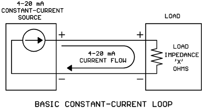
Basic constant current loop configuration

Before we discuss connecting multiple loads to a constant current loop, let’s get familiar with the basic constant current loop containing a single load:

On the left we have a constant-current source that is regulating the current to some desired value (the desired value is determined by a calculation in a controller, measured physical value in a sensor, etc.). The constant current leaves the source, flows through the load, and returns to the source.

Simple, right? What could go wrong? As usual, “the devil is in the details.”

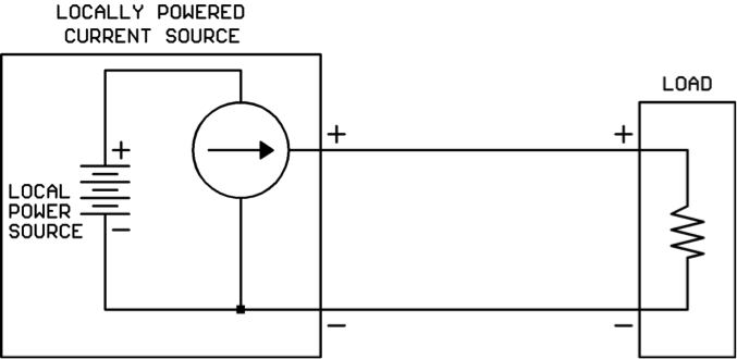
Two different styles of current sources

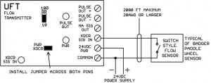
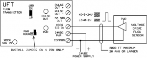
There are two different styles of current sources you should be aware of. We’ll call the first style the “locally powered” current source. It has its own source of power for the 4-20 mA output and the only other item needed to complete the loop is the load:

You will usually find this type of current source on the output of a powered controller.

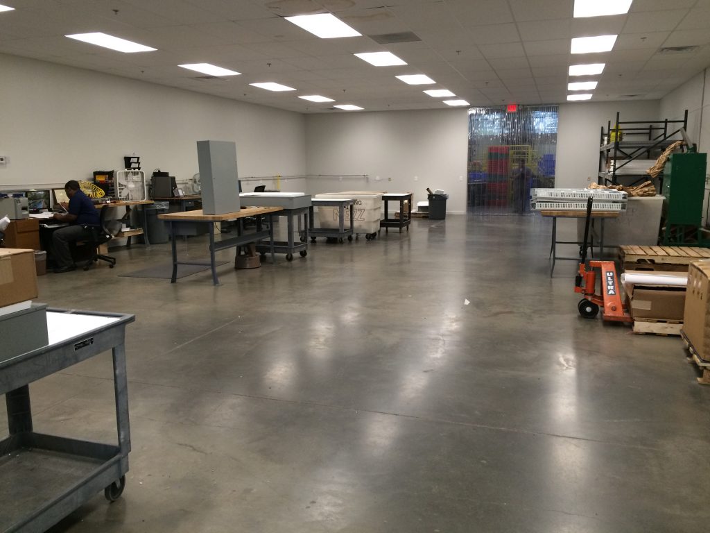
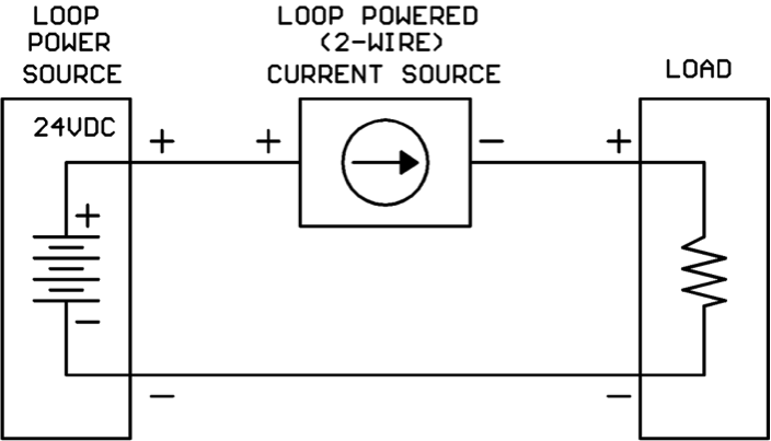
We’ll call the second style the “loop powered” or “2-wire” current source. It does not have its own power source built-in, but rather depends on a separate power source (usually 24VDC) wired into the loop:

You will find this type of current source in many 4-20 mA loop-powered temperature, pressure, and humidity transmitters.

Current sources have a “maximum load impedance” they can drive

Current sources like small values of load impedance, in fact they can drive their current straight into a short circuit (zero ohms load impedance)!

Current sources run into trouble when the load impedance gets too large. When the load impedance gets too large, the current source will not be able to make the higher values of current (near the 20 mA end) flow. The current value will plateau at some value less than the desired value.

How do I know the “maximum load impedance” my current source will support?

For a locally-powered current source, you will need to find the maximum load impedance value on the product’s data sheet.

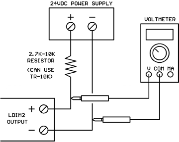
For a loop-powered current source, you may find a parameter called “maximum load impedance (with 24V supply)” on the data sheet. If you do not, you will have to perform the following steps:

1. Find a parameter called “minimum operating voltage” (or some very similar wording) on the current source data sheet.

2. Calculate maximum load impedance as follows:

Maximum load impedance = (Loop power supply – minimum operating voltage) / 0.020

For example, suppose we are using a 24V loop power supply and we see on the data sheet that the 2-wire current source needs a minimum of 11V to operate. Then we would calculate:

Maximum load impedance = (24V – 11V) / 0.020 = 650 ohms

Now that we know something about how a single-load constant-current loop works, let’s see what kind of complications we get into when trying to drive multiple loads!

Connecting multiple loads to the current loop

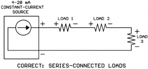
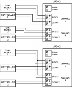
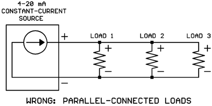
Rule #1: All loads must be connected in series around the loop, never in parallel.

Below are sketches of the right way (series) and the wrong way (parallel) to connect loads in a current loop:

currently figure 4

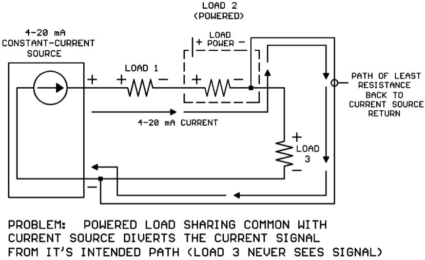
At first glance this requirement seems simple enough. That’s because we’ve drawn all the loads as 2-wire loads that don’t require power supplies. A not-so-obvious problem may occur if the loads do require power supplies. The current will always take the “path of least resistance” back to the current source whatever that path might be. If one of the loads before the last load has a power connection back to the current source, this connection will be the “path of least resistance” and the 4-20 mA will bypass the rest of the loads in the loop:

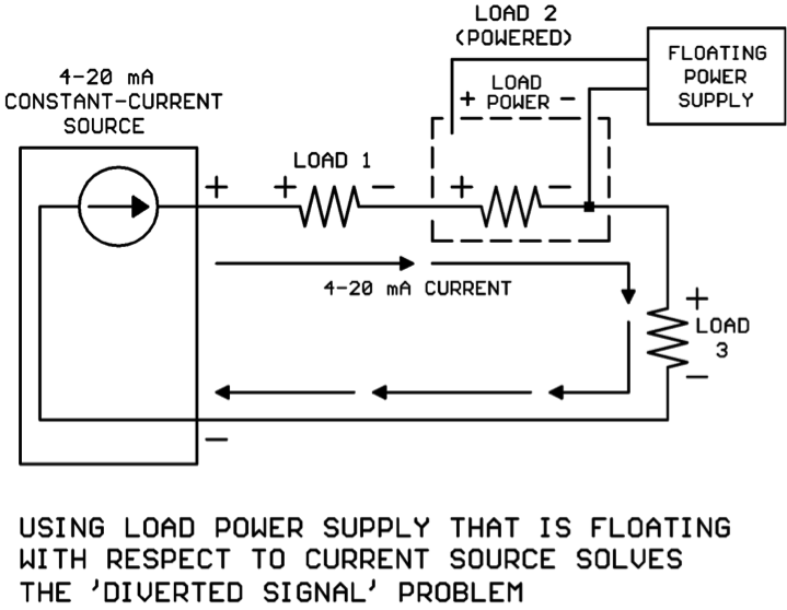
If the powered load is a standalone module, you may be able to use a dedicated “floating” transformer or small DC power supply to power the load and resolve the issue:

If multiple loads in the series connection are powered, each load would need its own power supply that is floating with respect to all the other supplies. For example, if Load 1 and Load 2 were both powered, Load 1 would need a power supply that is floating with respect to Load 2 and the current source, and Load 2 would need a power supply that is floating with respect to Load 1 and the current source. It can get messy quickly if there are several powered loads in the loop!

Consider also that If the powered load is a controller input and the controller is serving other inputs and outputs, it wouldn’t be practical to “float” the entire controller subsystem’s power connections.

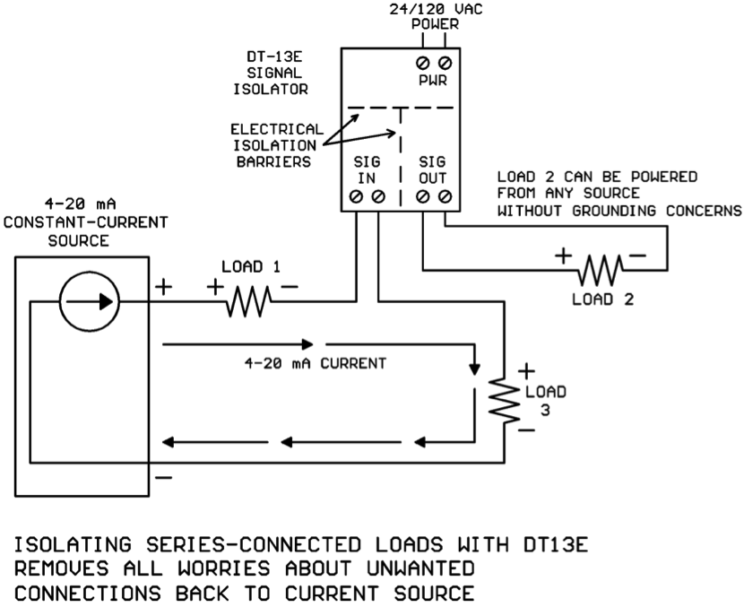
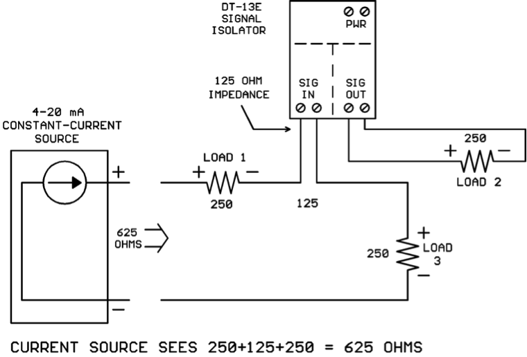
In cases where a floating power supply for each load is not practical, it’s time to employ a signal isolator module such as the DT-13E from Kele:

The DT-13E signal isolator has its inputs isolated from its outputs, and both inputs and outputs are isolated from the power terminals. So with the DT-13E installed, it just doesn’t matter where Load 2’s power source comes from, it will not corrupt the 4-20 mA current in the loop.

Rule #2: The sum of all the load impedances must be less than the maximum load Impedance the current source can support.

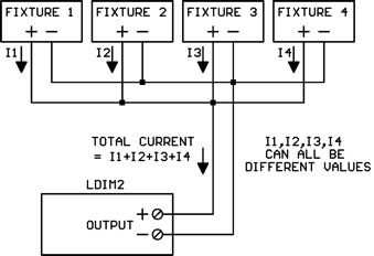
When the mA loads are wired in series (as they must be) the total load impedance seen by the current source is the sum of the individual load impedances. So if each of the three loads in the drawing below is 250 ohms, the total load impedance seen by the current source would be 250 + 250 + 250 = 750 ohms:

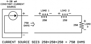
Suppose your current source data sheet shows that it can only drive 650 ohms maximum impedance? Houston, we have a problem…

What can you do if your total load impedance adds up to more ohms than the current source can handle? This is another way that the DT-13E signal isolator can sometimes help. Many HVAC 4-20 mA loads have impedances of 250 to 500 ohms, but the DT-13E mA input impedance is only 125 ohms. So by isolating one or more loads using DT-13Es, not only do you remove grounding concerns but you may also lower your total loop impedance to a value the current source can handle:

Now the current source only sees 250+125+250 = 625 ohms which is lower than its maximum load impedance, and Rule #2 is satisfied.

Conclusions

Multiple loads inserted in a 4-20 mA current loop must be connected in series. If the series-connected loads are powered devices, “sneak paths” between the load power supply connections and the current source may misdirect the 4-20 mA so that not all the loads receive the signal. Isolating the series-connected load with a DT-13E or similar signal isolator will solve this problem.

The sum of the series-connected load impedances may be too high for the current source to handle. The DT-13E signal isolator’s impedance of 125 ohms is less than that of many common HVAC loads. Isolating a load with the DT-13E may lower the total loop impedance to an acceptable value.

Shedding Some Light On 0-10V Dimmable Lighting Fixtures

Posted on April 14, 2015March 15, 2022 by Kele Inc

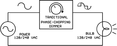
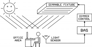
A very popular way to decrease energy usage these days is to use dimmable lighting fixtures and throttle back on the electrical lighting when outdoor light is available through windows or skylights. A light sensor such as the Kele MK7 family can feed light level information into a building automation system (BAS). The BAS can then use an intelligent algorithm to vary the electrical lighting level with changing outdoor light levels to maintain a constant level of indoor illumination while saving energy.

In order for the BAS to command the dimmable lighting fixtures to the desired light level, some sort of control interface must exist between the BAS and the light fixtures. There are several types of light dimming systems out there in the world with different control interfaces. The one we want to discuss today is known as the “0-10V current sinking” dimming system. We will also briefly mention several other types of light dimming systems, but they are not the focus of today’s article.

Classic Phase-Chopped High Voltage Light Dimmer System

The first light dimming system we’ll briefly touch on is the classic phase-chopping system. These dimmers connect in series with the high-voltage line to the lighting load and perform the dimming by removing part of each half-wave of the AC cycle:

This dimming system is typically limited to small-to-medium incandescent loads although some of the newer CFL and LED light bulbs will work with it also. These dimmers are typically manual-adjust units without any control interface to a BAS.

Networked Digital Light Dimming Systems

DMX is a networked digital light dimming/control system used in theaters and at rock concerts. DALI is a networked digital light dimming/control system that is popular in Europe and has found some use in the USA.

“0-10V Current-Sinking” Light Dimming System

This is the dimming system we want to discuss today. It is formally defined in the standard IEC 60929 Annex E.

Although the interface is named “0-10V” it’s not like the 0-10V analog interfaces we are accustomed to in the HVAC world! In the HVAC world the 0-10V is generated in the controller and is consumed by the load like this:

The classic 0-10V analog interface shown above is NOT the same as the 0-10V dimmable lighting interface! The “0-10V Current Sinking” lighting interface is implemented as shown in the following diagram:

Wow, that’s quite a bit different than what we are used to! The voltage source for the 0-10V signal is actually contained in the lighting fixture, not in the controller!

The voltage source is typically more than 10V, something in the 11-20V range. A series resistor located inside the lighting fixture allows the light dimmer module to “pull down” the original voltage to the desired value. The dimmer module does this by varying its own internal resistance until the desired voltage appears across its output terminals. Those of you who have studied circuit theory will recognize the combination of light fixture resistance and dimmer module resistance as a classic “voltage divider” circuit.

You will notice that a small current flows around the loop from light fixture to dimmer module and back to the fixture. The value of this small current is NOT the control signal, the voltage across the terminals is the control signal. The small loop current is just a necessary evil to make the voltage divider circuit work as needed.

Hmmm… I’m getting the idea that a standard 0-10V output from a BAS controller may NOT work with a 0-10V dimmable lighting fixture. Is that correct?

That is correct. Your 0-10V BAS output might work with a dimmable lighting fixture if you are very lucky. But probably, it won’t work. If you’re unlucky, you might burn up the 0-10V output on your BAS controller.

So… I need a specialized dimmer control to drive these 0-10V lighting fixtures. Where can I get such a dimmer control?

We’re glad you asked. J Kele sells the LDIM2 light dimmer module which is specifically designed to interface with 0-10V current-sinking dimmable lighting fixtures. The LDIM2 can accept standard 0-10V or 2-10V or pulse-width input signals from your BAS controller and provide the necessary current-sinking 0-10V output for the light fixtures. The 0-10V current-sinking output to the light fixtures is electrically isolated from the BAS signal inputs to prevent any interference between the two systems.

Can one LDIM2 dimmer module control multiple lighting fixtures?

Yes it can, just wire up the wire pairs from multiple lighting fixtures in parallel like this:

The total current flow through the LDIM2 output will be the sum of all the individual lighting fixture currents. Different makes and models of fixtures may supply different current values.

How many lighting fixtures can I attach to the LDIM2 output?

That depends on the control current flow from each lighting fixture. The maximum load current allowed on the LDIM2 output is 0.5 amps. So you can add lighting fixtures until the total from all the fixtures reaches 0.5 amps, but you can’t go further. If, for example, each fixture supplied 1 mA of current, you could attach 500 fixtures to one LDIM2 (0.5 amps / 0.001 amps = 500).

If you have so many lighting fixtures that the total control current exceeds 0.5 amps, wire them up in “banks” where each bank is 0.5 amps or less and is controlled by its own LDIM2 dimmer.

How do I find out how much current a particular model lighting fixture puts through the LDIM2?

The IEC 60929 Annex E standard specifies that the control current value should be between 10 uA (microamps) and 2 mA (milliamps). However, there’s absolutely no guarantee that the lighting fixture manufacturer adhered to these guidelines.

If you’re really lucky, maybe the lighting fixture data sheet will tell you the value of the control current. If you cannot find a published value for the control current, please don’t just assume a value. Also don’t mistake the lighting fixture’s supply current for the fixture’s control current. The fixture’s supply current will almost always be on the data sheet, but will be a much higher value, possibly several amps.

If you have access to the physical light fixture(s), you can measure the control current with your DC mA meter. Just put it across the two signal wires coming down from the fixture(s). But beware, the mA meter resistance is less than 1 ohm. It will pull the voltage down very close to zero volts, and the lights will go dark, so don’t do this during work hours on an occupied space unless the people are warned first!

What happens if the fixture wires are connected to the LDIM2 with the polarity reversed?

If the lighting fixture wire polarity is hooked up backwards, the voltage will go to about 0.7V which is near 0% light level. Nothing will be damaged, but the lights will go out.

How can I test the LDIM2 on my workbench if I don’t have a dimmable lighting fixture available?

You can use a standard 24VDC supply and a pull-up resistor like this:

The catalog description of the LDIM2 is “fluorescent dimming control.” Will it work with dimmable LED lighting fixtures?

Yes, it will work with any dimmable lighting fixture that uses the 0-10V current-sinking interface. You just need to figure out what control current the fixture puts through the LDIM2’s output so you don’t overload it by attaching too many fixtures.

Conclusions

The 0-10V current-sinking interface used by dimmable lighting fixtures is not compatible with the standard 0-10V outputs used in HVAC/BAS systems. You should use a specially-designed dimmer control module such as Kele’s LDIM2 for dimmable lighting fixture applications.