Contributed by Siemens
Hydronic systems are cooling and/or heating systems that utilize a liquid, such as water or mixture of water and glycol, as a heat transfer medium. The water is either heated or chilled and then circulated throughout a building to maintain comfort and temperature. Hydronic systems are specified in commercial buildings because of water’s thermal characteristics, as well as the availability, general safety, and ability of these systems to scale for larger buildings.
Principle hydronic systems elements consist of:
Generation elements – These elements are either the boilers to heat the water or chillers to cool the water. Cooling towers may also apply if waterside heat rejection is designed for the chillers (versus airside heat rejection).
Distribution elements – This includes the piping and pump network from the generation equipment out to each individual zone and/or space.
Consumption elements – These may be anywhere there is a heat transfer surface or coil. This includes air handling units, chilled beams, radiators, fan coil units, and variable air volume units.
Design Evolution
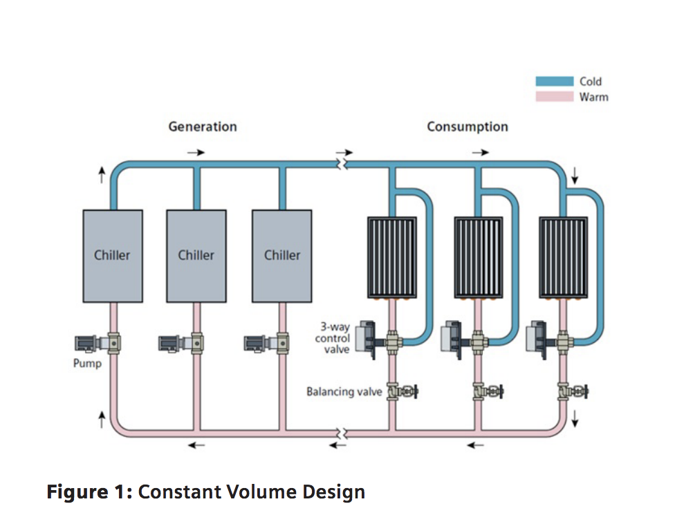
Older constant volume system designs use considerable energy compared to more modern methods because pumps see a relatively constant head pressure having to continuously pump water throughout the entire piping network. In the example shown in Figure 1: Constant Volume, the pumps are either on or off, and the chillers supply a constant volume or flow of water via distribution piping to our consumption side of the loop.
On the consumption side, air-side loads are transferred to the heat transfer coil, and flow is varied through the coil via three-way valves bypass to maintain load requirements. The total flow through the distribution mains, however, remains constant. A balancing valve is required to balance out the circuits to ensure proper flows to each load.
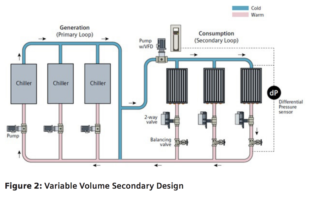
A variable volume secondary design (see Figure 2) distributes chilled water to the consumption coils that are decoupled from the generation or primary loop. The advantage is that a secondary pump is used with a variable frequency drive (VFD) to control flow, which allows a two-way valve to be used instead of a three-way valve at the consumption coils. The benefit of this design is that the pumping energy is greatly reduced to just the flows needed to each load. However, a balancing valve is still required to balance the secondary circuits.
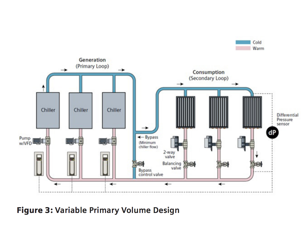
A variable primary volume design still maintains a generation or primary loop and consumption or secondary loop (see Figure 3). With this configuration, the chillers are selected so that they can unload with variable flow through the chillers. Each chiller gets its own VFD on its respective pump. The bypass now gets a control valve that effectively directs water into the consumption or secondary loop. The advantage of the variable primary volume design is that only what is needed is pumped through the chillers and the bypass control valve directs the flow to the consumption or secondary loop. The entire distribution piping network is seeing only the flow it needs when it needs it, effectively reducing any unnecessary head losses in the system. This allows a two-way valve to be used instead of a three-way valve at the consumption coils and a balancing valve will still be required to balance the secondary circuits.
Design Implications of Variable Flow
Three major impacts of designing for variable flow (both primary and secondary) are:
- Heat transfer efficiency at the coils (Treturn – Tsupply)
- Control valve selection, which in turn impacts pumps and associated VFDs and energy savings
- Staging of generation equipment such as boilers and chillers
Coil Heat Transfer Efficiency
Several factors can affect coil heat transfer efficiency, including dirty filters, coil fouling, and improper piping. From an operational perspective, because coils are designed for a certain flow, it is important to ensure that the coils are neither undersupplied (loads not met) or oversupplied (creating low delta T). As two-way control valves in variable flow systems open and close to meet associated loads, system pressure variations affect flow rates through the valves. This is initially addressed by statically balancing the system via manual balancing valves at coil locations for the nominal operating conditions. This can only be achieved, however, for one given ‘‘ideal’’ operating condition.
Overflow Effect on Coil Efficiency
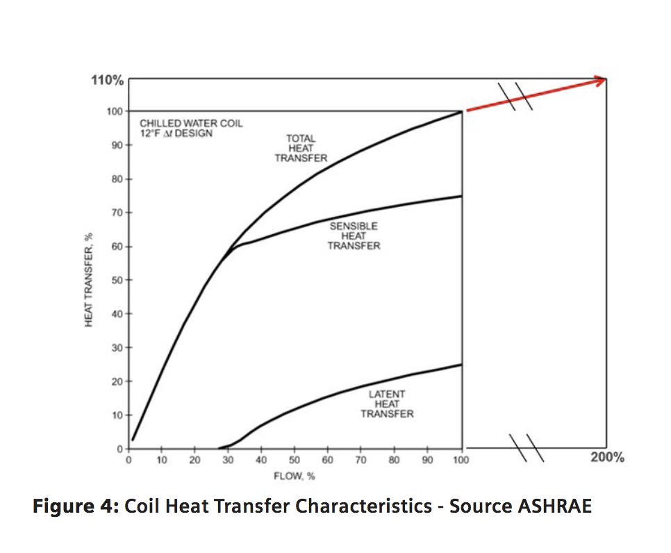
Coils can encounter overflow scenarios that lead to the erosion of system designed Delta T. The most common is overflowing the maximum limitation of the coil due to pressure fluctuations in the system or due to an incorrect understanding of those limitations, particularly in chilled water coils. As seen in (Figure 4) – a typical chilled water coil’s heat transfer curve plateaus out as it nears maximum flow. In general, if 200% flow is forced through the coil only 10% more heat transfer will take place. This can be a primary cause of delta T erosion as the extra flow will not pick up the additional heat due to coil design limitations. The impacts of delta T erosion at just a few of the heat transfer coils then can cause two negative systemic effects.
![]()
First, recall our waterside heat transfer equation stating that the heat transfer potential of our water is directly proportional to our flow rate (GPM) and our delta T (ReturnSupply temperature). As coils are overflowed in the system our delta T shrinks, effectively derating the rest of the coils within our system. As this starts to occur the control system may react by increasing flows across the system which will lead to further delta T erosion as the coils were selected at the initial delta T conditions. As more flow is required at this lower delta T to satisfy load conditions, our pumps are negatively impacted by the increase in energy used to circulate this additional flow. Second, in the case of chillers and heat pumps, overflow causes inefficiencies in the energy generators. Overflow of dedicated consumers can lead to a return temperature lower than the nominal design value in cooling mode and a return temperature higher than the nominal design value in heating mode. This decreases the energy efficiency of boilers and chillers by 2% and 3%, respectively, because a decrease of the evaporation temperature of a chiller below its design value by 1° decreases its performance by about 3%.
Dynamic-Balancing against Pressure Differences
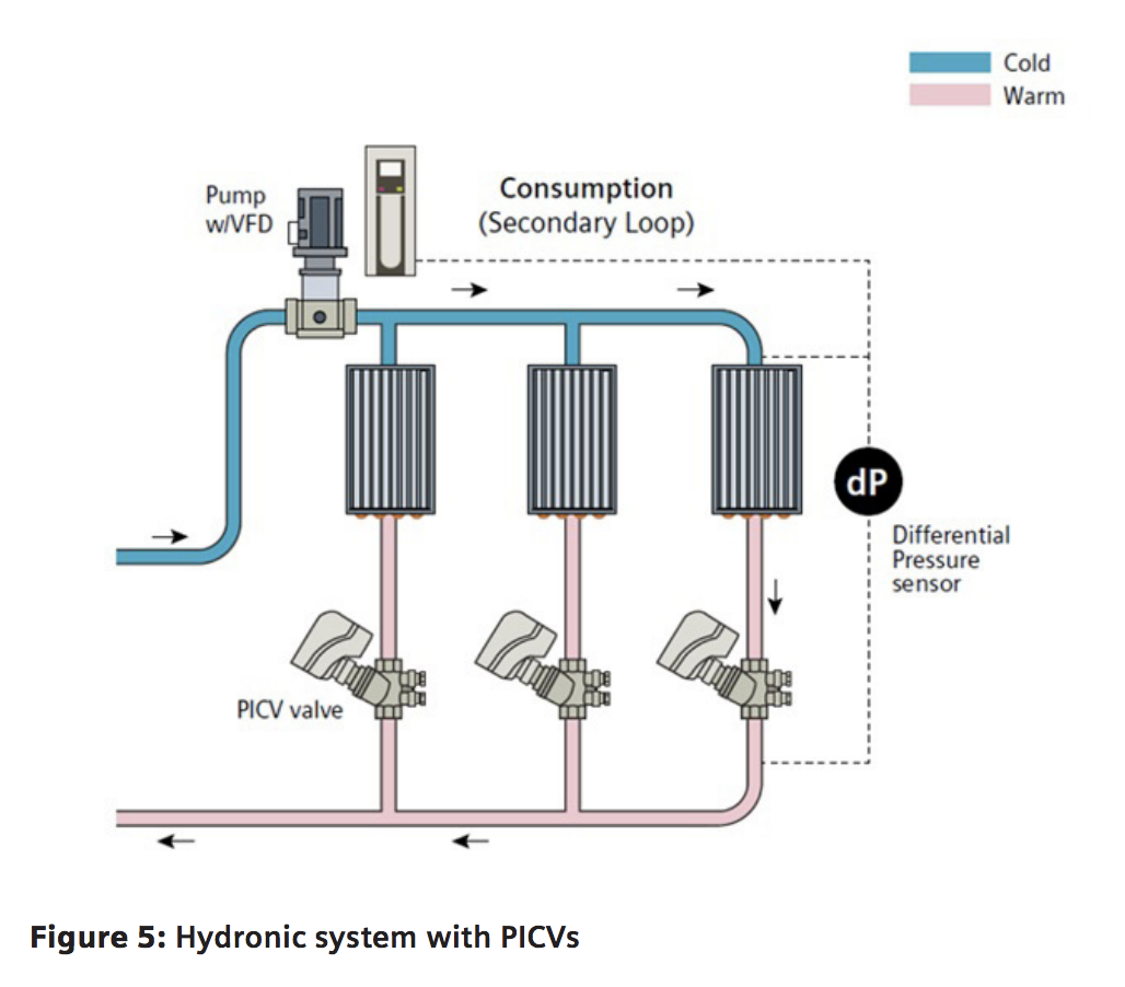
One way to address the inevitable pressure fluctuations in hydronic systems is with pressure-independent control valves (PICVs). Within their range of operation, PICVs are not affected by pressure fluctuations in the building’s hydronic system. This is called dynamic-balancing or auto-balancing.
This basic functionality is achieved by an internal differential pressure regulator working in series with the main flow control valve and regulating the pressure differential of the flow control valve using a pressure inlet and membrane. Hence, the flow across the entire device is independent of the pressure changes in the system, and flow is determined only by the travel of the control valve. When used with a terminal unit, PICVs ensure proper flow, optimizing heat transfer, and system performance. In heating and cooling applications, the auto-balancing function generates energy savings by:
- Eliminating heat exchanger overflow at any time and under any operating condition;
- Improving control accuracy by eliminating hydraulic pressure dependency between neighboring control loops; and
- Enabling advanced energy distribution strategies by eliminating the risk of heat exchanger starvation.
Variable Frequency Drive Considerations
Reducing the speed of pump motors using variable frequency drives (VFDs) lowers energy costs by reducing the amount of energy it takes to operate the pumps. A VFD often is specified to save money by reducing energy consumption in pumps or other motor loads that may be found in a typical building.
The following best practices provide engineers with information on how to specify a VFD to meet load conditions while achieving efficiency. To effectively specify a VFD, engineers must understand these key points:
- Load (operating power, torque, and speed characteristics)
- Duty cycle (percentage of operation at 100% load, 50% load, etc.)
- Desired benefits by using a VFD (energy savings, soft start, controllability, etc.)
Understanding the load is the first step to determining what can be gained by deploying VFDs. In building hydronic systems, the most common type of motor providing power to a load is a three-phase AC induction motor. For a given power rating, the motor base speed is inversely proportional to the effective torque rating for that motor. For example, selecting a 1,800 rpm motor instead of a 1,200 rpm motor reduces torque by one-third. Once a load’s starting requirements are determined, the next step is to look at the load’s running requirements. In building systems, excluding constant horsepower and constant speed/ torque loads, typical loads that can take advantage of VFDs are:
- Variable speed, variable torque (fans, blowers, and centrifugal pumps)
- Variable speed, constant torque (positive displacement loads, such as screw compressors, reciprocating compressors, or elevators).
To support a characteristic load, select a motor to meet a specific starting requirement and running output power, torque, and speed.
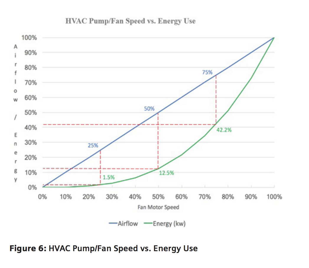
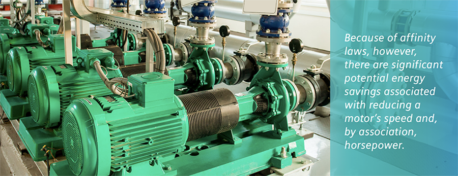
Because of affinity laws, however, there are significant potential energy savings associated with reducing a motor’s speed and, by association, horsepower. If we can define the required change in motor speed to meet the change in flow for a centrifugal load, the change in required power is proportional to the cube of the change in speed from one system point to another. The change in required torque is proportional to the square of the change in speed from one system point to another.
This nonlinear relationship between power and speed can be exploited for significant energy savings if the speed of the motor can be changed. For example, if the speed of the motor is reduced by just 5% from the full load, a realization of 14% energy savings is possible. When the speed of the motor is reduced to 80% from full load, 49% of energy savings can be realized. Every incremental slowdown of the speed of the pump becomes more valuable from an energy savings standpoint.
For centrifugal loads, there is potential to significantly increase energy efficiency by reducing motor speed.
The Hydronic System: Differential Pressure Control
As hydronic systems continue to evolve from constant volume systems to constant volume primary, variable volume secondary, and variable primary systems, it is important to maintain flow across all heat transfer circuits.
Because a VFD is connected to either the primary or secondary pumps in variable hydronic flow systems, the control loop will need an input to monitor and control. A differential pressure sensor located on the circuit most likely to be starved, also known as the critical circuit, is a common and reliable input configuration. The differential pressure sensor will allow the hydronic system to set a minimum pressure across the critical circuit, ensuring flow availability across all circuits.
The pump and variable frequency drive will take the differential pressure measurement across the critical circuit and control via the VFD’s onboard proportional-integral derivative (PID) controller, allowing the pump speed to be optimally reduced and maximize energy savings.
Contact Kele today or Chat with a technical representative here on kele.com if you have questions or need help finding a product.


